A
quick overview of SOFTWARE PACKAGES (and databases) used in evaluation
[this
document is available by clicking on HELP link in any of the Results pages]
The 2015/2016 EM
Modeling Challenge evaluation system includes software for preprocessing and
verification of models and their assessment at 4 levels of granularity: multimers, monomers, domains (if any) and inter-chain
interfaces.
Acceptance,
preliminary preprocessing and analysis of models:
·
Maxit
and other tools (Cathy Lawson - acceptance, preliminary preprocessing)
·
In-house scripts (Andriy Kryshtafovych –
analysis and preprocessing)
Multimers:
·
TEMPy
1-3
, (global and local model-map fit)
·
PHENIX 4, including a new module
for the EM model challenge implemented by Pavel Afonine
(used for analysis of global and local model-map fit)
·
EMRinger
5
(global and local model-map fit based on side-chain fit)
·
Model/Map match (using chain comparison
module of PHENIX)
·
QSscore
(Torsten Schwede /Martino Bertoni – not published yet; used for assessing multimeric model
fit to reference structure(s) )
·
EMRinger
·
LDDT scores on chain correspondences
found with QSscore (above)
Monomers
and Domains:
·
Molprobity
6 (verifying stereochemistry
of models)
·
dFIRE
7 *not sure we need
it – results are often inconsistent; new version - dFIRE2 is hard to get; Molprobity may be enough
·
PROSA 8 *not sure we need
it – results are length dependent, Molprobity may be
enough
·
ProQ
9 (one of the best
CASP single-model accuracy assessment methods)
·
QMEAN 10 (one of the best
CASP single-model accuracy assessment methods)
·
LGA 11 (used for
generating GDT-family based scores - main rigid-body superposition-based scores
used in CASP)
·
TM-score 12 (similar in
principle to GDT_TS, i.e., rigid body superposition based - widely used in protein
modeling community)
·
LDDT 13
(superposition-free measure; compares difference in distance patterns)
·
CAD score 14
(superposition-free measure; compares difference in contact areas)
·
ECOD 15
(database for extracting domain definitions)
·
Davis_QAconsensus
16 (in-house tool for
assessment of models based on their clustering)
Interfaces:
·
IFaceCheck
(Andriy Kryshtafovych, just developed; tool name is tentative)
TARGETS
Targets are numbered consecutively, from T0001 to
T0008. Target name is usually provided together with the target name, e.g. GroEL: T0003.
If different reference structures are used in a
specific type of evaluation, target ID will include PDB ID of the reference
structure, e.g. GroEL: T0003_1xck. Several reference
structures can be used for the same target. If chains with different
configurations are present in the target – the reference structure ID would
include chain name as well, e.g. GroEL: T0003_1svt_A
or GroEL: T0003_1svt_H.
If different EM maps are used in a specific type of
evaluation, map EMDB ID will be shown in a separate column of the evaluation
results. Results for different maps of the same target are organized as
different subtargets, e.g. target T0002 has two subtargets: one for the emd_5623 map and another – for
emd_6287.
MODELS
Information on submissions received at Rutgers is
available for organizers from the Google Docs spreadsheet https://docs.google.com/spreadsheets/d/12C4SUu9L37qvRBu0RCLoC4KgZXbcbYbpVn5q3TxACd8/edit#gid=0
The same table (with the columns containing
sensitive information being redacted) is publicly available from the Model Descr. Tab on the Results pages. Sub-tables with the
information on the submitted models for each target are accessible by clicking
on any model name in the Model column of any target-specific Results Table.
Each submission has its own name as assigned by the
PDB extract system (e.g., emcm102_GSec – see column B of the spreadsheet). This
name is used only internally and does not appear in the evaluation tables.
If several models are provided in the same
submission file, they are preliminary split into separate files. Each model is
assigned a unique ID and is evaluated separately.
Model names that are used in the Results tables
(e.g. T0003EM164_1) are formed according to the following scheme:
·
T0003 [target name]
·
EM [electron microscopy]
·
164 [predictor number (see below)]
·
_1 [model number from this predictor for
this target]
Note
1: The suggested target reference structures and all models were analyzed one
by one for their format consistency and compliancy with the evaluation
software. Problems were recorded in a separate file available from the Google
Docs.
https://docs.google.com/document/d/1lJnq4Yv0ZOYUS6hffp3o2d_41KVNwlave47ktJdZ_MQ/edit
The
most typical problems were identified and systemized in yet another Google Docs
document:
https://docs.google.com/document/d/1CehhkMVmKBkLxIc3tmoinNjajRHPHqDtEwdzSnMy9Yw/edit
Note
2: If a model is submitted as a monomer and symmetry info is provided within
the model, the assessors may consider applying the symmetry operators and
evaluating the model not only as a monomer, but also as a multimer.
PREDICTORS
Each group participating in the EM Model Challenge
is assigned a unique number. Predictor IDs corresponding to each model are provided
in the column C of the spreadsheet. The group_ID – group_name correspondence is concealed from the assessors
and available only to the organizers.
Description
of the EVALUATION MEASURES and the WEB INFRASTRUCTURE
 Results
of the evaluations are presented in the EM Model Challenge Results website (http://model-compare.emdatabank.org/,
see the screenshot below). Each target has its own Results webpage that can be visited
by clicking on the target pictograph/name. Submitted models in plain text
format can be accessed by following the “Repositorium
of models” link at the top of the page. Models are grouped in folders by target;
directories ending in “_” contain representative chains from multi-chain
submissions; directories ending in “–Dx” contain
models split in structural domains, if any. Directory ‘fixed’ contains models
fixed by the submitters or organizers. The final Results tables contain results
for the fixed models and not the original ones.
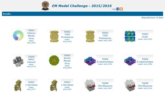
Results pages hierarchy.
Once in any of the
Results pages, you can switch between targets through the “Target” drop-down
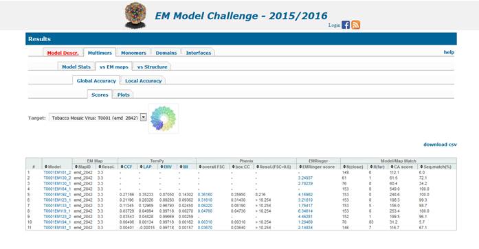
menu at the target-specific pages (thick blue arrow in the screenshot below).
 Each
model is evaluated at four levels of its structural composition: quaternary
structure, tertiary structure, constituting domains and inter-chain interfaces
(if applicable). Input data and evaluation tools are different for different
assessment approaches. The results are reported separately under four different
tabs provided at the highest level of the Results page hierarchy: Multimers (i.e. quaternary structure), Monomers (tertiary
structure), Domains, and Interfaces. Additionally a Model Descr
Tab is available to provide information on the details of the submitted models
(as provided by the predictors). Going down the hierarchy users can browse
results of specific analyses. Data are available as sortable result tables, clickable
bar graphs or scatter plots (details further in the text).

![]()
1.
Multimers (top level tab in the
evaluation infrastructure)
Multimer
prediction models are evaluated in three regimes:
1.1) Model Stats
1.2) vs the experimental EM map (and/or versus the
improved map, if submitted together with model) and
1.3) vs the experimental
structure(s).
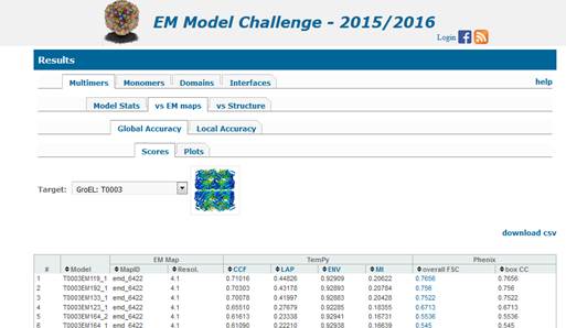
Results in each of the evaluation modes are
presented under a separate tab (pointed to by the blue arrow below).
![]()
1.1.
Assessment of stereo-chemical properties of the multimeric models (2nd
level tab “Model Stats”) is carried
out with the PHENIX 4
module designed specifically for the EM model challenge. This type of
evaluation does not require reference structures. The results are presented as
tables (3rd level tab Scores) and histograms (3rd level
tab Histograms).
1.1.1. Scores.
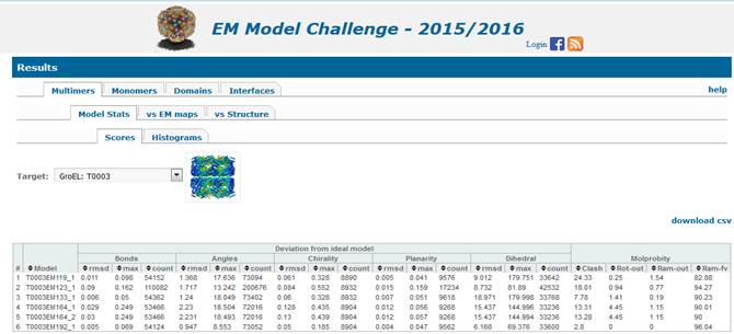
Left section of the results table under the Scores tab (above) reports deviation of
·
Bond distances,
·
Angles,
·
Chirality,
·
Planarity
·
and Dihedral angles
from
the values observed in ideal models. For each of the listed model features,
three values are provided: 1) rmsd calculated on the selected features, 2) maximum value of the deviations (in
the selected feature units, e.g. Angstroms for Bonds and Degrees for Angles), and
3) and number of the selected
objects in the model.
Right section of the table reports Molprobity scores for the whole multimeric model:
·
Clash-Score: the number of all-atom
steric overlaps > 0.4Å per 1000 atoms.
·
Rot-out: Rotamer
Outliers score - percentage of sidechains conformations classified as rotamer outliers, from those sidechains that can be
evaluated.
·
Ram-out: Ramachandran Outliers score -
percentage of backbone Ramachandran conformations classified as outliers.
·
Ram-fv:
Ramachandran Favored score - percentage of backbone Ramachandran conformations
in favored region.
Note
that scores for separate chains are provided under the Monomers evaluation tab.
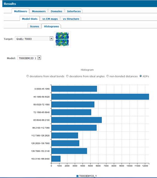
1.1.2. Histograms.
Histograms pages provide binned distribution of some
of the model geometrical features for the same ranges of the scores for all
models (so they are directly comparable). User can pick four different
histograms per model showing:
·
deviations from ideal bonds,
·
deviations from ideal angles,
·
deviation of non-bonded distances,
·
atom
displacement parameters (ADPs).
X-axis shows number of examples in bins specified in
y-axis.
1.2. Evaluation of multimeric models vs the maps (2nd level tab “vs EM maps”) includes calculation of global and per-residue fitness measures generated with TEMPy 1-3
, PHENIX 4 and EMRinger5. All three packages have been locally installed and tested.1.2.1. Global
(full-model) fitness (3rd level tab Global Accuracy)
1.2.1.1. Global
scores reported in the table (4th level tab Scores) are:
From
TEMPy:
·
CCC: cross-correlation function to score
goodness of fit between the original map and the map convoluted from the model
coordinates to the author-specified resolution of the experimental map (or an
updated user-provided map)
·
LAP: Laplacian-filtered CCC
·
ENV: Envelope score
·
MI: Mutual information score
Please read the paper [2] for a more
detailed explanation of TEMPy scores.
From
PHENIX:
·
overall FSC: overall model-map Fourier Shell
Correlation
·
Box CC: overall map-model
cross-correlation score (per chain scores are available by clicking at the
score)
·
Resolution at the FSC=0.5
From
EM Ringer:
·
EMringer
score (clicking at the score will bring up the plot of the EMRinger
score for different Electron Potential Thresholds).
There is a strong correlation
between resolution and the EMRinger score. This is to
be expected, given that EMRinger score reports on
side chain density, which is only resolvable above about 4.5 Å. In general, for
maps above around 3.5 Å resolution, the minimum score
that should be expected is around 1, with a benchmark for a very good score
lying around 2. Most structures which have been carefully refined, either in
real or reciprocal space, score above 1.5, with some structures getting scores
above 3.
Model/Map
Match (PHENIX module chain_comparison):
·
N(close) - number of Cα within 3Å
·
N(far) - number of Cα further than 3Å
·
CA score - the number of Cα within
3Å of the target divided by the rmsd
·
Seq. match % - percentage of Cα atoms
that have the correct residue name
1.2.1.2. Global
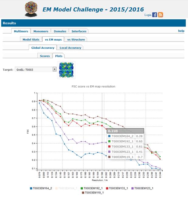
fitness plots (4th level tab
Plots) are:
·
FSC curves built from the PHENIX results
for all models evaluated on the specific target (see below). This page is also
reachable by clicking on the FSC score in the table of results. Mouse over the
graph shows data values for each curve for the selected resolution value
(x-axis). Mouse over the model name (under the graph) highlights the line for
the selected model (can be very useful if many lines are running very close to
each other). Clicking on the model name turns the line invisible (and greys the
group name); clicking on the grey model name makes the line visible again.
1.2.2.
Local
(per-residue) fitness (3rd level tab Local Accuracy)
Per-residue fitness of models to electron maps is shown
as a Summary table and Interactive line plots.
1.2.2.1. Summary tab.
Summary
table shows TEMPy’s CCC score and PHENIX’s box CC
score for each chain in the model.
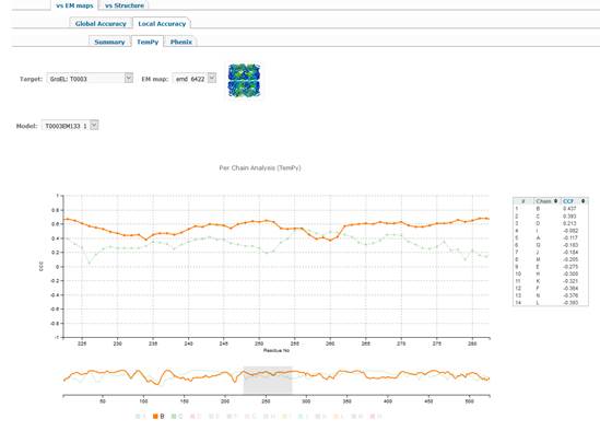
1.2.2.2. TEMPy tab.
·
TEMPy
tab provides access to scatter plots based on the SMOC calculation (Segment
Based Manders’ Overlap Coefficients - please read
paper [3] for a more detailed
explanation). The per-residue accuracy of models according to this score can be
explored in more details by selecting a specific region in the model on the
lower line-only graph. Click on the residue you want to start a detailed
exploration, drug mouse to the end of the desired interval and then release
(alternatively use mouse’s scroll wheel for this operation) – the top plot will
change accordingly showing details for the selected region. By default, the
plots are shown for the chain with the best overall CCC score (highlighted at
the bottom of the plot). If you want to see plots for some other chains on the
same graph – please click on the additional chains that are greyed out at the
bottom of the graph by default. (the exemplary plot
below shows graphs for chains B and C selected). Moving the mouse over the names
of the selected chains will highlight respective lines in the plots above.
Scores for all chains from the model are shown in the table to the right of the
plot.
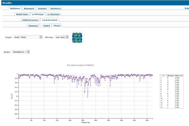
1.2.2.3. PHENIX tab.
·
Per-residue graph for the chain with the
highest box CC score. The per-residue accuracy of models according to this
score can be explored in more details by selecting a specific region in the
model on the lower line-only graph. Click on the residue you want to start a
detailed exploration, drug mouse to the end of the desired interval and then release
(alternatively use mouse’s scroll wheel for this operation) – the top plot will
change accordingly showing details for the selected region. By default, the
plots are shown for the chain with the best overall box CC score (highlighted
at the bottom of the plot). If you want to see plots for some other chains on
the same graph – please click on the additional chains that are greyed out at
the bottom of the graph by default. Moving the mouse over the names of the
selected chains will highlight respective lines in the plots above. Scores for
all chains from the model are shown in the table to the right of the plot.
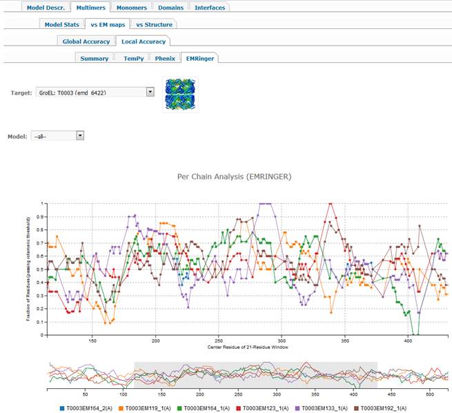
1.2.2.4. EMRinger tab.
·
Per-residue graph showing fraction of
residues passing the rotameric threshold. Selecting
option ‘–all--‘ in the Model dropdown menu will
visualize the first (alphabetically) chain for all the models submitted on the
selected target. The graphs can be explored in more details by selecting a
specific region in the model on the lower graph (using the technique described
above). If a specific model is selected (instead of –all-), then graphs for all
chains in this model can be visualized. By default, the plot is shown for the 1st
alphabetically chain. If you want to see plots for some other chains on the
same graph – please click on the additional chains that are greyed out at the
bottom of the graph by default. Moving the mouse over the names of the selected
chains will highlight respective lines in the plots above.
1.3. Evaluation of multimers
vs the reference structure (2nd level tab “vs Structure”) is carried out using a newly developed QSscore (Quaternary Structure score) from Torsten Schwede’s group. The
software is locally installed and tested. The package first finds the best
mapping between the reference target and model chains using the structure
symmetry, and then reports 4 scores:
·
QS_best:
the fraction of interchain contacts (Cβ-Cβ<12A)
that are shared between two structures for best fitting interface
·
QS_global:
the fraction of interchain contacts that are shared
between two structures for all interfaces
·
RMSD calculated on the whole aligned
structure (CAs of all common chains)
·
LDDT (Local Distance Difference Test): non-symmetric
measure that does not penalize for overprediction,
e.g. a tetrameric model (containing a perfect dimeric model) vs the dimeric target
is giving a LDDT score of 1.0 (check paper [13] for more info on
the LDDT)
2.
Monomers. Submitted models are first split into separate
chain-based models, which are then checked for similarity, and all different
chain-based models are evaluated separately.
Monomer accuracy assessment is carried out with
three types of measures: single-model validation measures; model consensus
measures and comparison to the reference structure (X-ray or/and EM).
Single-model validation measures do not require a
'ground truth' structure and include knowledge-based potentials (Molprobity and dFIRE) and CASP
a-priori estimators of global and local model accuracy (ProQ
and QMEAN – all locally installed and tested).
Comparison to the reference structure is made with
both, superposition-free measures (including LDDT and CAD) and rigid-body
superposition-based measures including RMSD, GDT_TS, GDT_HA
(sequence-dependent, i.e. assuming one-to-one residue correspondence in model
and target), LGA_S and TM-score (sequence-independent, i.e. finding alignment
first). All packages are locally installed and tested.
If several models are submitted on the same target,
overall and local consensus of models is checked with locally implemented DAVIS-QA
method. Global and local similarity of models is calculated in terms of GDT_TS
score and distances between the corresponding residues in models. Models with
the highest level of conservancy get the highest reliability scores.
Calculations in this regime include all-against-all models scores, so in
principle any of the models can be used as a reference structure.
2.1. Results of global
accuracy assessment (2nd level Global Accuracy tab) are
presented in form of sortable tables (tab Scores) and plots (tab Plots)
2.1.1. Global
accuracy scores.
Table for global accuracy scores include:
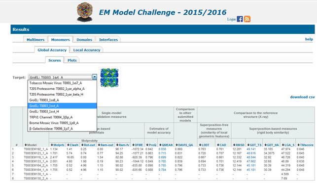
Single-model
validation measures:
five
scores from Molprobity (see Molprobity
paper from the 1st page of this manual for details):
·
Molprb:
aggregated Molprobity Score calculated according to
the formula: Molprb = 0.426 *ln(1 + Clash-Score) +
0.33 *ln(1 + max(0, Rot-out - 1)) + 0.25 *ln( 1 + max(0, (100 - Ram-fv) - 2 )) + 0.5
(note: the lower score - the better model; scores below 3
indicate likely stereochemically reasonable model)
·
Clash-Score: the number of all-atom
steric overlaps > 0.4Å per 1000 atoms.
·
Rot-out: Rotamer
Outliers score - percentage of sidechains conformations classified as rotamer outliers, from those sidechains that can be
evaluated.
·
Ram-out: Ramachandran Outliers score -
percentage of backbone Ramachandran conformations classified as outliers.
·
Ram-fv: Ramachandran
Favored score - percentage of backbone Ramachandran conformations in favored
region.
·
dFIRE:
an energy-based score, i.e. the lower (negative) - the better. Note: The new version of dFIRE
score has been published this year, but the software is not publicly available.
I tried to get it through personal contacts – was promised, but guess the
software is not in a form ready for the distribution).
·
ProQ:
a score from an a-priori estimator of model accuracy; the score is scaled to
0-1 range with higher numbers corresponding to likely better models (see the ProQ2
paper for details on the sequence and structure-based features used in scoring)
·
QMEAN: a score from an a-priori
estimator of model accuracy; the score is scaled to 0-1 range with higher
numbers corresponding to likely better models (see the QMEAN paper or http://swissmodel.expasy.org/qmean/cgi/index.cgi?page=help
web page to learn about 6 scoring function terms contributing to QMEAN).
Model
consensus method:
·
Davis-QA: a score showing average
similarity of the selected model to all other submitted models on this target
in terms of GDT_TS (range 0-100)
Reference
structure superposition independent measures:
·
LDDT: the score evaluates similarity of
inter-atomic distances in model and targets (see the LDDT paper for details).
The score is scaled in the range 0-1.
·
CAD: the score evaluates protein models
against the target structure by quantifying differences between contact areas
(see the CAD paper for details). The score is scaled in the range 0-1.
Reference
structure rigid body superposition-based methods:
·
RMSD: rmsd on
all CAs
·
GDT_TS (Total Score): = (GDT_P1 + GDT_P2
+ GDT_P4 + GDT_P8)/4, where GDT_Pn denotes percent of
residues in model that can be fit to target under the distance cutoff of nÅ (see the LGA paper for details). GDT_TS is scaled in the
range 0-100. Note: Clicking on the GDT_TS
value for the model will show GDT plot, which is also accessible from the Plots
tab.
·
GDT_HA (High Accuracy): a fine-grained
version of the GDT_TS score with halved cutoffs: GDT_HA = (GDT_P0.5 + GDT_P1 +
GDT_P2 + GDT_P4)/4, where GDT_Pn denotes percent of
residues in model that can be fit to target under the distance cutoff of nÅ. GDT_HA is scaled in the range 0-100.
·
LGA_S (0-100) is similar to GDT_TS, but uses
weighted scores from the full set of distance cutoffs in [0-10] range. Unlike
GDT_TS, can be used in situations, where alignment between model and target
cannot be established based on sequence.
·
TMscore:
a measure that is conceptually similar to GDT_TS, but has a different score
normalization procedure; TM-score is in the range (0,1],
where 1 indicates a perfect match between two structures (see the TM paper for
details).
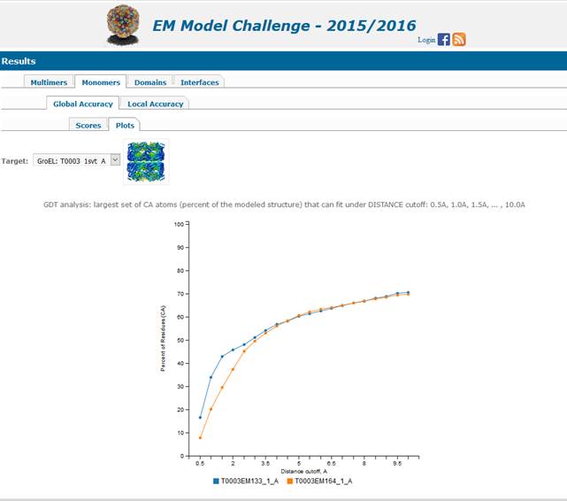
2.1.2. Global
accuracy plots.
Accuracy of the model versus the reference structure
is visually summarized by GDT plots showing percentage of residues in the model
that can be superimposed into the target under the specified residue-residue
distance cutoff. The closer the curve stays to the y-axis – the better the
model. An ideal model would be represented by a curve going straight up and
then staying horizontally across the whole range of distance cutoffs. Graphs
are interactive so the lines in them can be switched on and off and the
underlying scores can be shown using the techniques described in section
1.2.1.2.
2.2. Results of local
accuracy assessment (2nd level Local Accuracy tab) are presented
in form of combined bar plots and tables.
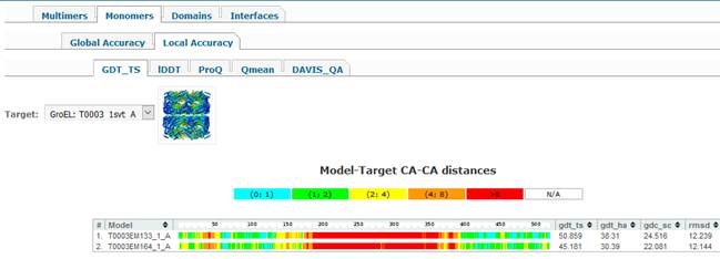
There are five tabs under
the parent Local Accuracy tab, each corresponding to the selected evaluation
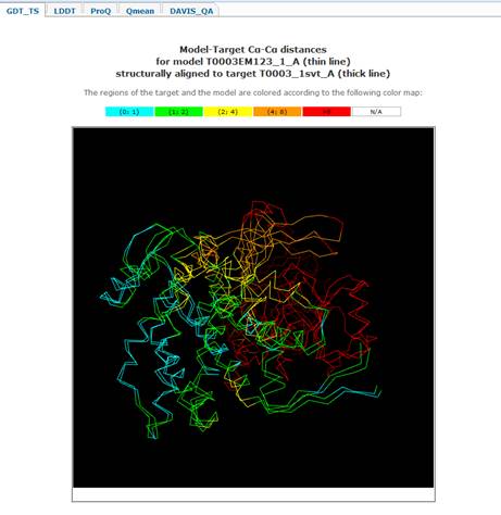
measure (GDT_TS, LDDT, ProQ, QMEAN and Davis-QA). Clicking
on each of the tabs shows color-coded bar showing per-residue accuracy of the
model according to the selected score. For example, clicking on the GDT_TS tab
shows CA-CA distances between corresponding residues in model and target after
their optimal superposition, while clicking on the
LDDT tab gives per-residue LDDT score (type of the score is specified in the
plot title). Clicking on the color-coded bar shows structural superposition of
model and target colored the same way as the underlying bar.
3.
Domains. If monomeric units consist of several structural
domains the models are evaluated at the level of domains for different
reference structures, if needed. Targets are split into domains by consulting
the DomainParser and DDomain2 software and the ECOD
database of structural domains.
General principles of web infrastructure
for Domain results is similar to the Monomer
infrastructure.
4.
Interfaces
We locally developed the software for identification
of corresponding interfaces, and calculation of statistical measures on
interface similarity. First, similar interfaces are clustered in the target and
model based on the Jaccard distance between them
(identity of residues constituting interface). Clicking on the interface name
(e.g., AK, meaning interface between the chains A and K) in the column
Corresponding Interfaces shows the full list of similar interfaces in the
cluster below the table (see below).
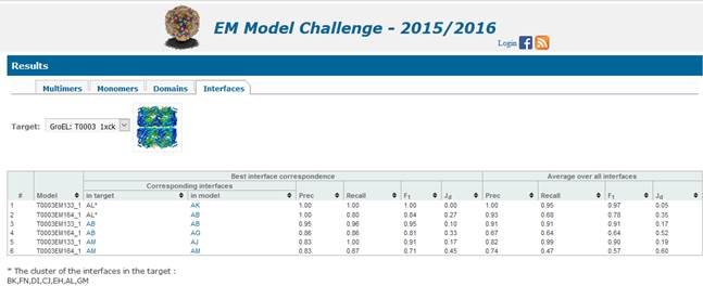
For each pair of similar interfaces, we calculate
·
Prec
(precision) = TP/(TP+FP)
·
Recall = TP/(TP+FN)
·
F1-score = 2*Prec*Recall/(Prec+Recall)
·
Jd
(Jaccard distance) = (FP+FN)/(TP+FP+FN)
·
between
interchain contact pairs in target and models. The
scores are reported for the best scoring interface from each of the
corresponding interface clusters and also as average from all pairwise scores
from all interfaces in the cluster (right side of the table).
·
RMSD between the residues belonging to
target interfaces and corresponding residues in the model is also calculated
together with the
·
Coverage of the target by the models
residues (percentage of target residues used in the rmsd
calculation).
References: